
RAMYA SRIDHAR – APRIL 20TH, 2023
In Spring of 2022, I took the Econ 100B Macroeconomics course with Raymond Hawkins. I found it to be a very enlightening course with an engaging curriculum. Observing the course alone, disregarding professor ratings or execution formatting, the material is very interesting, and forms the basis of a lot of economic thought. Even for those pursuing microeconomics, observing and learning about macroeconomics may be a worthwhile endeavor, just for the additional insight and perspective it can provide.
Keep in Mind…
It’s important to note that this course has a lot of formulas, and a lot of derivations. Picture 10th grade algebraic proofs? Kinda like that. The Problem Sets can be challenging if you’re unfamiliar with Excel or other data computation mediums, but between the student discord and the offered resources, most areas of uncertainty are generally made navigable.
One of the things I found most interesting about this curriculum is that almost every idea introduced in this course is accompanied by a formulaic/mathematical definition, and a broader theoretical explanation. This dichotomy really helped in establishing the significance of these new ideas as formulaic variables and as tangible concepts we can see and encounter in everyday life. Acknowledging both the algebraic position and contextual realities of these variables is very important to doing well in this course.
This course is a great introduction to the intersection between Economics and public policy. If your interests lie in public Economics, you might find this course to be more interesting. This course just really helped in understanding the larger gears of the market, especially as it relates to the government or fiscal policy.
Here’s a breakdown and walk through of the actual subject material. (Note: This is a brief rundown of what I considered to be the central bullet points of the course; not everything will be mentioned.)
The Curriculum
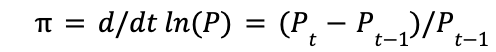
One of the first and most important ideas we encounter in this course is the National Income Identity: Y=C+I+G+NX. In this equation, we see the four main categories of spending represented by the variables on the right, and the GDP on the left (Y). On the right, we see Consumption (the spending of domestic households on final goods and services), Investment (the spending of new capital goods and inventory investment), Government spending (the spending by the government on goods and services), and Net EXports (Exports – Imports). This is one of the basic ways to measure national income, and we refer to this formula consistently throughout the course. It’s a basic idea that forms a foundation upon which the rest of the content is based. Related to GDP, it is also important to note the 3 major price indexes—the average level of prices for some designated goods and services, relative to the prices of that good during a select base year—GDP deflator, the Personal Consumption Expenditure (PCE) Deflator, and the Consumer Price Index (CPI). These all deal with another extremely important variable that is crucial to this course—inflation, represented by . The equation for inflation is simple:
The variable appears in a number of equations used in this course, including the Fisher Equation:

In this equation, the variable r represents the real interest rate, the variable i represents the nominal interest rate, and 𝝅^e represents the expected inflation. Essentially, the Fisher Equation is to project ex-ante real rates based on expected inflation. In finance, it becomes a mechanism for investors to compensate for (high) inflation.
In economics, the ideas of inflation and unemployment are always inextricably linked. One of the central themes of Economics is the concept of the Phillips Curve. In Econ 100B, we expand on this.
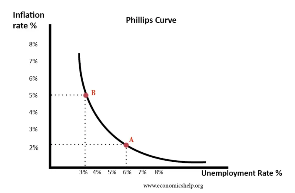
The Phillips curve is a graphical representation of the relationship between unemployment and (wage) inflation. It holds that inflation and unemployment have an inverse relationship—an increase in one leads to a decrease in the other. This relationship is vital in understanding a lot of economic principles and ideas. Looking specifically at wage inflation vs. unemployment, we see that the Phillips curve fundamentally identifies a supply and demand relationship; when the supply of labor is lowered (unemployment rate increases) the price of labor increases (wage inflation).
When gauging unemployment, it’s important to note the various Measures of Unemployment:
- the Unemployment Rate = Unemployed/Labor Force,
- the Participation Rate = Labor Force/ Population, and
- the Employment Ratio = Employed/Population
(For this course, these three formulas serve as easy points on the midterms and the final. It’s very useful to memorize these early on. Generally speaking, they’re much easier to understand relative to the rest of the course.)
The Phillips curve also seeks to explain the relationship between inflation and output. Paired with Okun’s Law, which asserts that unemployment and output share an inverse relationship, we get new equation for the Phillips curve:
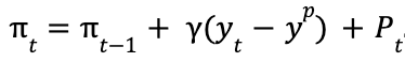
The specifics of the variables aren’t that important now, but basically, this equation provides insight into sources of increased inflation—whether it’s a demand problem or a supply problem or both. This equation becomes very relevant in comprehending the course material.
Another formula we end up using repeatedly is the Cobb-Douglas Production function, modeled:
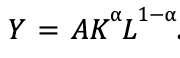
This may appear more complicated in structure, but the ideas behind it are simple once you understand their utility. In this equation, Y is economic output, A is total factor productivity—defined as the proportion of output to input meant to measure efficiency; K is capital stock—the value of capital input that is used to produce Y; L is labor—the amount of human capital it takes to produce Y; and the alpha value simply represents the allocation of funds to capital, where 1-alpha is the amount that goes to labor. From the Cobb-Douglas Production Function, we obtain the Growth Accounting Formula, or
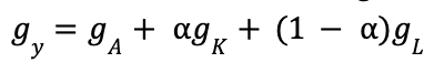
We find this by calculating the natural logs and derivatives of the CB function. This formula is useful, as it reveals sources of growth and changes in growth for an economy over time. It also demonstrates how different economic structures have different reasons for growth.
Econ 100B deals with many economic models—one of the more prominent ones is the Solow-Swan Model. In short terms, it’s an economic model that projects long term economic growth. It expands on the Cobb-Douglas function to include savings rate, capital depreciation rate, and the labor force growth rate. This new hybrid equation is:
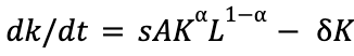
in which s is the fraction of output that is saved, and δ is the constant rate of capital depreciation. Essentially, this equation is just taking the Cobb-Douglas equation and adding real world factors to the calculations—the fact that capital depreciates, and that some amount of output is saved.
An important, new variable in this model is kappa (κ), which represents normalized capital, or capital per labor per worker efficiency. (This variable also becomes central to understanding the rest of the course, so it’s important to practice interpreting this variable both formulaically and contextually.) From this value, under the Solow-Swan model, we can find the Steady State Solution to the capital accumulation equation. Essentially, at steady state, there is a κ* value that, should the economy generate κ* amount of capital, it will stay at that level. Basically, steady state is the point in which kappa doesn’t change.
Another model that has prominent importance in the curriculum is the Romer Model. This model has more contextual importance than it does mathematical. The Romer Model, also referred to as the Endogenous Growth Theory, is a model in which labor is allocated between goods/services (L_p) and new technology (L_E). In simple terms, the Romer Model emphasizes the importance of investing in R&D; it postulates that the economy sees greatest growth when pioneering technological advancements and innovative ideas.
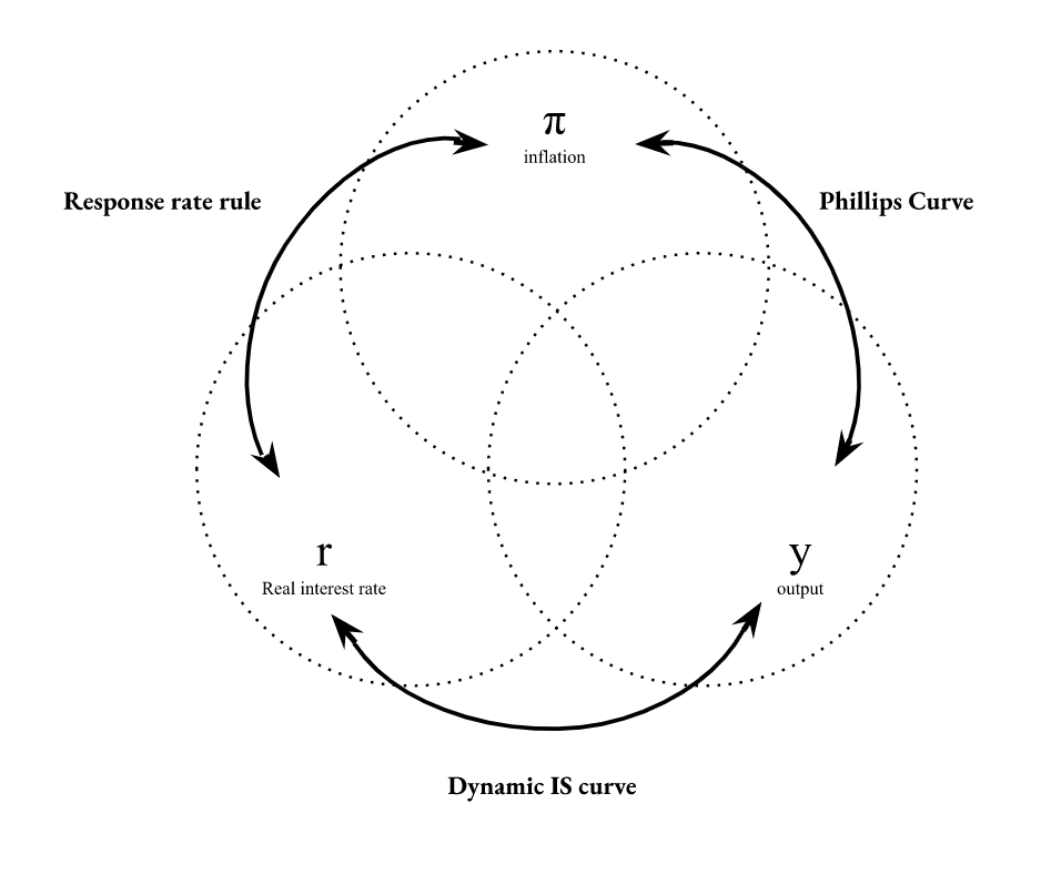
An important relationship that exists in Macroeconomics is the one between real interest rates and inflation. Interest rates exist to curb demand by increasing the cost of debt. In that sense, they are positively correlated with inflation–when we see high inflation, the Central Bank increases interest rates in order to rein it in. The optimal rate rule is an equation that determines the optimal real interest rate based on inflation, among other factors. We see expansionary policy when the actual interest rate is less than the optimal interest rate, and contractionary policy when the actual interest rate is greater than the optimal interest rate. This also becomes relevant when studying the IS curve.
The IS curve represents the inverse relationship between planned spending and the real interest rate. The IS curve is based on the principle that actual expenditures, or the total output, is equal to planned expenditures, or aggregate demand. It’s short form is represented by the equation
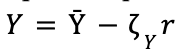
which is used to build the dynamic IS curve, represented by
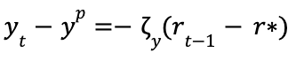
(Again, there are a lot of equations in this course, and thereby a lot of mathematical proofs and some degree of memorization.) The relevance of these are better understood in the context of the course.
Three central variables we repeatedly refer back to in this course are inflation, interest, and output. These represent the three prongs in the contextual venn diagram that represents this course. It’s especially important to identify and understand the relationship that exists between these three ideas.
In the last segment of the course, we run through several conceptual ideas—quantitative easing, the quantity theory of money, the law of one price, the relevance of behavioral economics in it all—but one of the prominent ideas that emerge is Sahm’s Proposal.
Many economists agree with the concept of cash transfers straight from the Central Bank as a way to stimulate demand. However, due to execution errors and public stigma against perceived ‘handouts’, cash transfers have always suffered in implementation. Obviously, consumer spending is an extremely important component of a functioning economy. A reduction in consumer spending can lead to unemployment and decreased output production. Sahm’s proposal was essentially a proposed stimulus package that would stabilize the economy by boosting consumer spending. Claudia Sahm observed that, everytime the three-month national unemployment rate rose by at least 0.50 percentage points relative to its low in the previous 12 months, the economy entered a recession. This detection technique was labeled the Sahm signal—she postulated that anytime the Sahm signal was triggered, automatic lump-sum stimulus payments would be made to individuals. All adults would be paid the same amount, with an extra 50% for each dependent an adult may have. This idea is very important for the course—it represents an innovative solution published recently (2019) to a long-standing problem. Hawkins uses this proposal to make the argument that innovation isn’t a gate-keeped field—with the proper research, innovation can be done by anyone, anywhere. (This can also pop up on the final, so it’s important to know the details!)
Overall, Econ 100B is a very interesting course. The first half can be pretty formula and math heavy, but the second half definitely leans theoretical. However, for Macroeconomics, a good balance is needed between the two. This course offers a solid foundation for understanding basic economic principles. In that sense, it’s definitely worthwhile.
Disclaimer: The views published in this journal are those of the individual authors or speakers and do not necessarily reflect the position or policy of Berkeley Economic Review staff, the Undergraduate Economics Association, the UC Berkeley Economics Department and faculty, or the University of California, Berkeley in general.