JEFFREY SUZUKI – FEBRUARY 11TH, 2020 EDITORS: ABHISHEK ROY & ODYSSEUS PYRINIS
For every avid student of history, the inevitable question of “what if?” tortures the mind. Winston Churchill called them the “terrible ifs”—alternate universes where the US was able to outlaw slavery through gradualist means or where Napoleon decided against his doomed invasion of Russia. However, historians often condemn such fantasies as being intellectual hogwash since practically every speculation made is unprovable. As historian Richard J. Evans opined, “In the effort to understand [history], counterfactuals aren’t [of] any real use at all.”
It should be obvious that many who engage in hypothetical history can often have some outstandingly banal and offensive questions such as “what if the Japanese were bat-bombed instead of nuked?” as one Japanese American Tufts student unfortunately encountered at a hypothetical history club. However, due to the rise of econometric methods, we argue that wholly dismissing hypothetical history is steadily becoming an outdated stance.
Instead, there now exists an abundance of public and private data available for use and, sometimes, for abuse by scheming economists. For instance, the World Bank provides data for over a thousand indicators for almost every country in the world. Merely querying a country on OurWorldinData.com yields information for hundreds of different criteria ranging from life expectancy and average schooling to the number of heads of cattle in the country. Instead of dismissing “what if?” hypothetical history as a waste of time, economists now have the data and tools to estimate hypothetical history. This estimation has a term in economics: “counterfactual.”
There are a number of ways to answer this “what if?” question. In 1994, the famous study on minimum wage by David Card and Alan Krueger popularized an econometric methodology known as “difference in differences.” Their paper analyzes the effect of New Jersey’s minimum wage increase on unemployment. They quantify this effect by using Pennsylvania as a counterfactual. Economists have adopted the nomenclature of “treatment” and “control” groups; in this case, New Jersey, undergoing the treatment of a minimum wage increase, serves as the treatment group while Pennsylvania serves as the control group.
However, a problem is encountered when considering that Pennsylvania and New Jersey are not identical in a number of respects, including unemployment before treatment, population, culture, history, and a plethora of other factors. In other words, Pennsylvania does not serve as a perfect counterfactual. Card and Krueger craftily solve this issue by making a crucial assumption: the differences in unemployment between Pennsylvania and New Jersey would remain the same if New Jersey did not pass its minimum wage law. This assumption is known as the “parallel trends assumption.” Hence, the methodology is called “difference in differences”—there is an initial difference before treatment and a difference after treatment. We take the difference in these differences. With this methodology, Card and Krueger found that the minimum wage law in New Jersey actually had a statistically significant negative effect on unemployment rates, a result that contradicts the conventional economic wisdom that higher minimum wages cause higher unemployment rates.
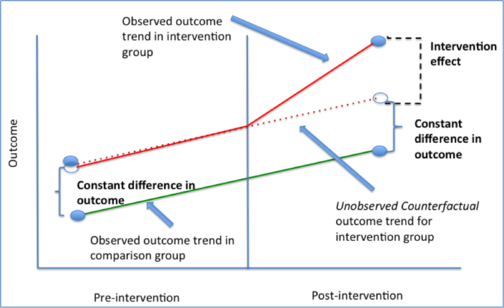
Visualization of parallel trends | Photo courtesy of Columbia University
Despite the initial controversy of the study, the difference in differences methodology has become a staple in economics to suggest causality. However, there is one potentially fatal flaw with this method: the parallel trends assumption is inherently unprovable. That is, it is impossible to see whether the differences between New Jersey and Pennsylvania would have indeed remained consistent over time without the increase in minimum wage. However, this is not the only methodology to estimate counterfactuals; the next one essentially creates a counterfactual.
In 2001, seven years after Card and Krueger’s study, a new methodology arrived to generate counterfactuals: synthetic controls. To estimate the economic effects of terrorist conflict in the Basque Country in Spain, Alberto Abadie and Javier Gardeazabal composited a number of Spanish regions to create a synthetic Basque Country which was compared to the real Basque Country. To create this synthetic Basque Country, Abadie and Gardeazabal collected data on several predictors of economic growth (e.g. years of schooling, trade openness, etc.) from every region in Spain. The general idea is that the synthetic Basque Country would have very similar predictor values as compared to the real Basque Country. In the end, they created a synthetic control that was 85.08% Catalonia and 14.92% Madrid, finding that the terrorist conflict in the Basque Country reduced GDP per capita by about 10 points relative to its synthetic control. For those interested, the full details of the mathematics can be found in their paper.
Both of these modeling tools may appear complex to the recreational reader of economics; therefore, we will provide a quick demonstration of both. The Berkeley Economic Review has already published an article providing accounts of the economic effects of regime change in Latin America. Thus, we will pick one country and ask: “what would the Nicaraguan economy look like if it had not gone through its insurrection in 1978?” The insurrection in Nicaragua was known for its ferocity, killing an estimated 50,000, roughly 2% of its population. Historians may dismiss this question as being a load of malarkey and an example of counterfactual history; however, as economists, we do not possess such reservations and will proceed regardless.
Using Difference in Differences:
We collect economic growth data from all Central American countries from the World Bank. We place Nicaragua in our treatment group and place the remainder of Central American countries in our control group.
We use the following difference-in-differences model:
GDP growthi=α+b(insurrect)i+c(time)i+δ(insurrecti • timei)+εi
Here, insurrect is a dummy variable. A dummy variable is a variable that equals 1 or 0, depending on how it is identified. In our model, we define our insurrect variable as being 1 in countries where insurrection occurred.
Meanwhile, time is also a dummy variable signaling when our GDP growth rate occurred; 0 denotes before treatment and 1 denotes after treatment. Finally, insurrect*time is also a dummy taking on the value of 1 when insurrection and time are both equal to 1. This is our treatment accounting for the effects of the insurrection. Put simply, the insurrect*time variable answers the following question: how is our GDP growth variable impacted when we observe Nicaragua after treatment? In our regression model, the subscript i merely denotes time period.
To perform the regression using our dataset, we use a statistical software called STATA. All of the variables used in the regression are defined in a .csv file or Excel file before importing the data into STATA. We obtain all of our data on GDP growth per annum from the World Bank.
After importing the dataset into STATA, we code as follows:
generate treat = insurrect*time
regress gdpgrowth insurrection time treat if inrange(year,1976,1979)
Here, we compress our insurrect*time variable into a single variable called “treat” so that we may utilize it in our regression along with the aforementioned variables defined in our regression model above.
STATA provides us with the following regression output:
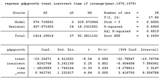
Note: Data for Central American countries and growth rate from the World Bank (2019) | Results by Jeffrey Suzuki
Looking at the regression output, “Coef.” stands for “coefficient” and represents the coefficient for the dummy variables in the model indicated earlier. This is essentially the insurrection’s effect on economic growth rates in Nicaragua. Under P>|t| (known as p-values), we can observe that the p-value under “treat” (denoting our treatment effect) is 0. For those who have not heard of the term “p-value,” it is the probability that the value we received for our coefficient is purely coincidental or, in other words, due to chance. A p-value of 0 implies, with near certainty, that the insurrection caused the decrease in economic growth. As a point of reference, p-values of less than 0.05 are usually considered statistically significant since it is the threshold at which statisticians consider the outcome beyond chance or luck.
An appropriate question that should be asked is whether our natural controls are actually valid. That is, do other Central American countries actually serve as suitable natural controls? Due to the unverifiability of our parallel trends assumption, this is unfortunately unprovable. However, we can make our findings more robust by using a second methodology: synthetic controls.
Using Synthetic Controls:
To create a synthetic Nicaragua, we collect data on the economic predictors of growth from neighboring regions, replicating Abadie and et. al. Due to the unavailability of some data, we can only use the following four predictors: GDP per Capita, Schooling (mean years of schooling), Openness to Trade (exports plus imports as a percentage of GDP), and Investment Rate (percentage of GDP in the form of capital investment). We obtain all of the data from the World Bank, except for mean years of schooling, which we obtain from Our World in Data.
So, how do we generate our synthetic control? Luckily, there is a package available for STATA that does this for us: Synth.
In order to install this package, we input the following code:
ssc install synth, replace all
Then, after importing our dataset, we define the panel data that we will use by declaring the unit of observation and the time:
tsset country year
Finally, we arrive at the most unintuitive part. At this point, we simply input our parameters in the format laid out by the authors of the package to generate our synthetic variable:
synth GDPpercap schooling trade_openness investrate GDPpercap(1968) GDPpercap(1970) GDPpercap(1975), trunit(1) trperiod(1977) xperiod(1968(1)1976) nested allopt fig
This is a lot to absorb, so to briefly explain:
- Synth is the command that we installed from our package.
- GDPpercap is our desired output. Schooling, trade_openness, investrate, and GDPpercap(X year) are all pre-treatment characteristics or predictors of economic growth
- trunit(1) denotes our treatment unit (Nicaragua is our first country which we labeled 1 in our dataset)
- trperiod(1977) denotes when treatment begins. In our case 1977 is the final year before the insurrection.
- xperiod(1968(1)1976) denotes the range of pre-treatment years that we want to cover with our synthetic control
- nested and allopt are optional parameters that increase the rigorousness of our synthetic control at the cost of extra computing time
- fig generates a chart comparing our synthetic control to Nicaragua.
Running this command in STATA yields the following results:
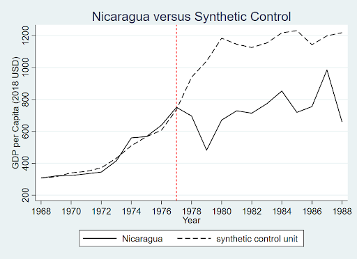
Note: Data from the World Bank (2019) and Our World in Data | Graph by Jeffrey Suzuki
As we can observe, our synthetic control maps on quite well with Nicaraguan GDP per Capita prior to insurrection. After 1977, the two diverged radically, suggesting that the insurrection was quite devastating. In fact, we can observe that Nicaragua does not “recover” (or converge with its synthetic control) from the insurrection for 10 years after the insurrection’s start in 1988. 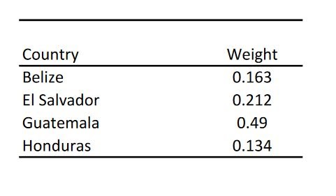
Note: Data from the World Bank (2019) and Our World in Data | Table by Jeffrey Suzuki
Synth also displays the weight of each country used in our synthetic control. Intuitively, countries with higher weights resemble Nicaragua more in terms of our economic predictors. In this case, Guatemala accounts for almost half of our synthetic control because it most resembles Nicaragua in the dimensions of schooling, GDP per capita, openness to trade, and investment rate.
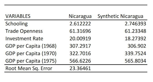 Note: Data from the World Bank (2019) and Our World in Data | Table by Jeffrey Suzuki
Finally, Synth also compares Nicaragua to our synthetic control along the predictors of economic growth which were defined earlier. As we can observe above, our synthetic Nicaragua is very similar to our real Nicaragua along every characteristic we specified in our code.
These are just a couple of methodologies out of several that could infer causality. It is important to note that no economist would claim that these methods are perfect. However, these tools serve as a means to make the case for causality.
If there is any redeeming characteristic of economics, it is that economists ask many questions across a plethora of topics. With the rise in prevalence of econometric methods, economics has made a steady transformation from a largely ideological and theoretical field to a more scientific, rigorous, and empirical one. Historians have correctly concluded that the past cannot be upended and changed to fit our fantasies. However, unlike historians, economists view these dreamy speculations of counterfactuals as a useful exercise that can be estimated. With the development of more econometric tools and methods and with the continued collection of data, economics has the potential to be a powerful tool to shape historical narratives by estimating the alternative histories we cannot observe with the naked eye.
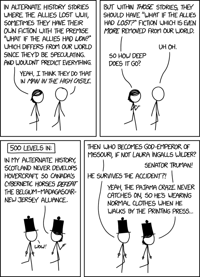
Featured Image Source: XKCD
Disclaimer: The views published in this journal are those of the individual authors or speakers and do not necessarily reflect the position or policy of Berkeley Economic Review staff, the Undergraduate Economics Association, the UC Berkeley Economics Department and faculty, or the University of California, Berkeley in general.